Since the Acoustic Influence Map (AIM) modeling tool was introduced with the launch of the OmniScan™ X3 flaw detector, it has become an integral assistance tool for the design of total focusing method (TFM) scan plans. AIM provides an estimate of the TFM acoustic intensity coverage for different TFM wave sets and scatterer types, enabling you to create a scan plan that maximizes the probability of detection (POD).
With the release of MXU 5.10, you’ll benefit from three major upgrades to AIM that further enhance the capabilities and ease-of-use of the OmniScan X3 and X3 64 scan plan tool.
1. Support for 3D Inspection Geometries
Previously, AIM only supported linear probes for which the TFM inspection area is directly below the primary axis of the elements. Now with the MXU 5.10 update, AIM supports Dual Linear Array™ (DLA) and Dual Matrix Array™ (DMA) probes for planar, circumferential outside diameter (COD) and axial outside diameter (AOD) geometries. This change is enabled by a major overhaul of the fundamental framework of the AIM model.
The updated AIM model provides similar results to some other commercial acoustic simulation software packages. For example, compare the below images generated by the updated AIM model and the sensitivity map obtained from CIVA 2021 (developed by CEA LIST) for the L-L TFM wave set on an AOD geometry.
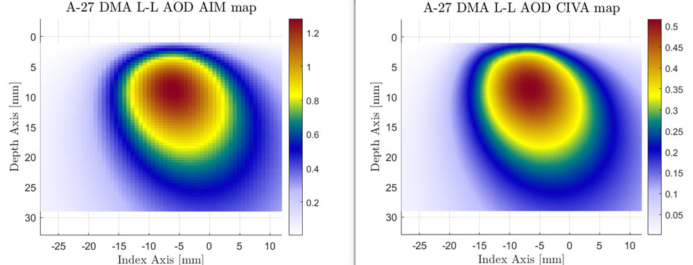
A27 probe AOD geometry comparison in L-L mode, AIM model (left) vs. CIVA software (right)
For this test case, the configuration included a 4DM16X2SM-A27 probe and a SA27-DN55L-FD25-IHC-AOD10.75 wedge on a pipe measuring 10.75 in. OD (273.05 mm OD). As you can see, the updated AIM model and CIVA 2021 model provide nearly identical maps for the DMA probe on this AOD geometry.
2. Improved Accuracy in the Probe’s Near Field
A second benefit of the overhauled AIM model is better simulation accuracy in the near field of the probe. Since the improved accuracy is more evident with contact inspections, a single element contact transducer was used to prepare the example images below. The size of the element is 1 mm × 10 mm, and the center frequency is 5 MHz.
These images show the single element near-field response of the previous and improved AIM models compared against the exact Rayleigh numerical model. The exact Rayleigh model is constructed by summing contributions from 100,000 uniformly distributed point sources on the surface of the single element.
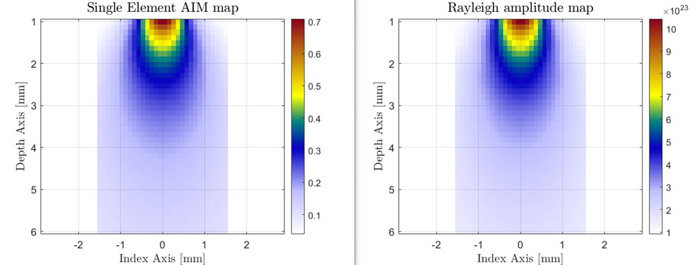
Improved AIM vs. Rayleigh exact model for single element transducer in L-L mode
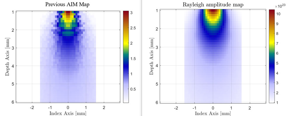
Previous AIM vs. Rayleigh exact model for single element transducer in L-L mode
Note the similarity between the improved AIM model and the Rayleigh model even at an observation distance of 1 mm (0.04 in.) from the element surface. In contrast, the previous AIM model has oscillations in the near field, which might affect the accuracy of near-field contact mode simulations.
3. Normalized Sensitivity Index
Before MXU 5.10, the sensitivity index of AIM was in arbitrary proportional units that could only be used to compare relative sensitivity between different wave sets. Now, we have rescaled the sensitivity index to provide a more intuitive interpretation of the sensitivity of a scan plan. In the next section, you can learn about the calculations that the MXU software performs to generate the sensitivity index for each AIM map. Later, however, you’ll find some concrete examples that will show you how to interpret the normalized sensitivity index and apply it practically.
Calculating the AIM Sensitivity Index’s Theoretical Maximum
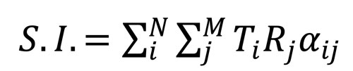
The sensitivity index corresponds to the maximum amplitude value in an AIM map. For each pixel, the amplitude is determined by 3 components (the transmitting response, the receiving response, and the scattering coefficient):
(1)
Here are the definitions for equation (1):
- N is the number of transmitting elements and M is the number of receiving elements.
- Ti the transmitting response from the i-th transmitting element. A maximum value of 1 represents perfect transmission. In other words, the transmitted intensity at the pixel is the same value as the intensity at the face of the transmitting element.
- Rj the receiving response from the j-th receiving element. A maximum value of 1 represents perfect reception. In other words, the scattered intensity is perfected received at the face of the receiving element.
- αijrepresents the scattering coefficient from the i-th transmitting element to the j-th receiving element. A maximum value of 1 represents perfect scattering. In other words, the incident intensity at the pixel is perfectly scattered into the receiving direction.
Equation (1) shows that the theoretical maximum value for the sensitivity is NM if there are N transmitting elements and M receiving elements. However, this value would not be reached in typical TFM setup configurations.
Sensitivity Index Differences for Planar and Spherical Scatterer Types
As with previous versions of AIM, AIM in MXU 5.10 supports both “spherical” and “planar” scatterers. In the updated AIM model, the spherical scatterer is treated as an ideal point scatterer where the incident intensity at the pixel is perfectly scattered into the receiving direction. In other words, αij has a value of 1 for all combinations of transmitters and receivers.
The planar scatterer in AIM is modeled as a circular void of 3 mm in diameter. The scattering coefficient αij is a complex function of the frequency as well as the normal, incident, reflected and observation vectors in 3D space. Here is a schematic drawing showing these vectors:
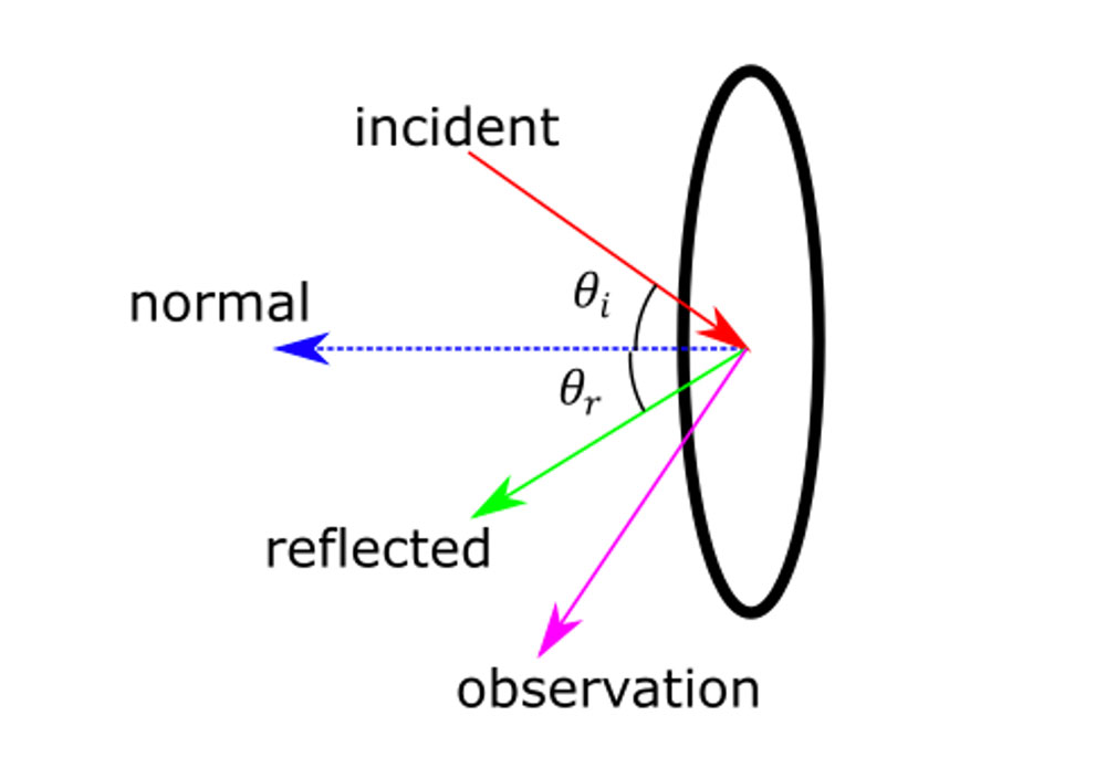
Schematic of normal, incident, reflected, and observation vectors for a circular void
For the circular void, the reflected angle θr would be equal to the incidence angle θi if there isn’t mode-conversion at the surface of the directional scatterer. Note that the observation vector may not lie on the plane formed by the normal, incident, and reflected vectors.
For this type of scatterer, the maximum αij value of 1 is reached if the incident, reflected and observation vectors are all coincident with the normal vector. This would be the case in pulse-echo mode if the transmission and reception beams are perfectly perpendicular to the directional flaw. Since the value of αij is 1 for only a special subset of Tx/Rx combinations, in general, the sensitivity index for AIM maps for a planar scatterer would be lower than the corresponding sensitivity index for an ideal spherical scatterer.
How to Interpret and Compare the AIM’s Normalized Sensitivity Index
Examples of AIM maps and their sensitivity indices for three different configurations using the same 5L32-A32 linear probe are provided in this section. Below each example you’ll find an explanation on how to interpret them.
For the first configuration, the probe is used in contact L-L mode, the corresponding AIM map for a spherical scatterer is shown here:
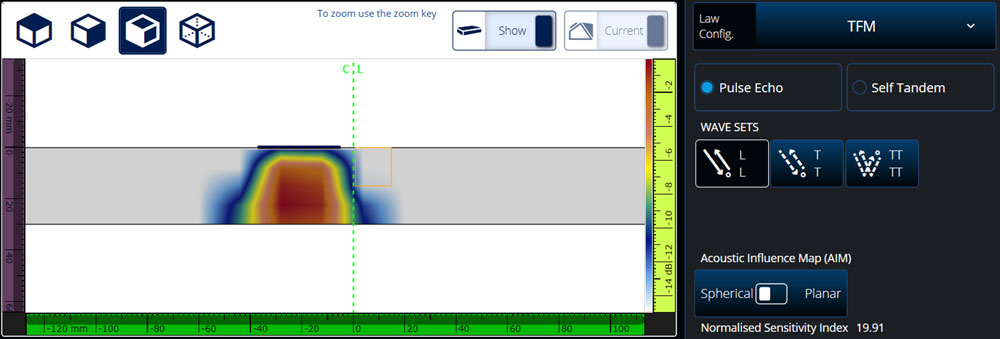
Configuration 1: Contact L-L mode spherical AIM map (sensitivity index = 19.91)
For this configuration, the normalized sensitivity index is 19.91 even though the theoretical maximum value is 1024 (32 transmitting and 32 receiving elements). The deviation from the maximal value is mainly due to element directivity and geometric beam spread.
For the second configuration, the probe is coupled to a SA32LS-N55S-Group D wedge and is used in T-T mode for COD geometry. The outside diameter of the pipe is set to 10.75 in. (273.05 mm). The corresponding AIM map for a spherical scatterer is shown here:
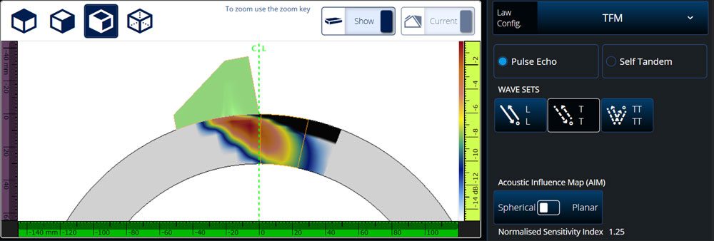
Configuration 2: COD T-T mode spherical AIM map (sensitivity index = 1.25)
In this AIM map, you’ll notice that there are some black pixels near the OD surface directly in front of the wedge. These black pixels indicate at least one acoustic path cannot be traced from an element to the pixel because of the physical boundaries of the wedge. Note that the sensitivity index is now 1.25, which indicates an additional 24 dB of gain is needed to have the same expected flaw amplitude level as the previous contact configuration. The decrease in sensitivity index is mostly due to increased geometric beam spread and complex refraction coefficients at the wedge/part interface.
The third configuration is the same as the second, but this AIM map is for a planar reflector:
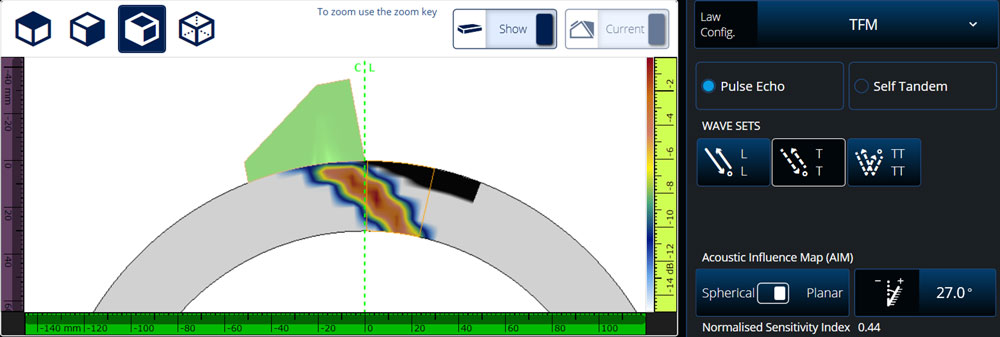
Configuration 3: COD T-T mode planar AIM map (sensitivity index = 1.25)
The flaw angle was set to 27° so the flaw’s normal is mostly perpendicular to the main beam propagation direction. Even with the optimal flaw orientation, the sensitivity index for the planar scatterer is only 0.44. The sensitivity index is lower than the previous map’s level of 1.25 because perfect perpendicularity between the flaw surface and the beam propagation direction cannot be achieved for all combinations of transmitting and receiving elements.
You can go to our Software Downloads page (and scroll down to “OmniScan”) to update to MXU 5.10 and start benefitting from these new AIM upgrades.
Related Content
White Paper: TFM Acoustic Influence Map
Frequently Asked Questions about TFM
Bookmark This! Access Our Total Focusing Method (TFM) Resources in One Convenient Location
Frequently Asked Questions about Phase Coherence Imaging
Get In Touch