Executive Summary
In all manufacturing processes there are limits to the surface topographies that can be produced. These limits can be represented in part by crossover scales. Understanding these scales is important for selecting process variables in additive manufacturing (AM), and for designing tooling for AM that can improve surface textures. This case study evaluated the measured topographies on surfaces made by an AM process for polymers. Multi-scale analyses of length and area, and their derivatives with respect to scale, were used to find crossover scales where the nature of the topography changes. Multi-scale analysis utilizes techniques designed to construct uniformly valid approximate solutions, both for small and large values of independent variables.
At sufficiently large scales manufactured surfaces can appear to be smooth. At sufficiently fine scales they appear to be rough (Brown, 2000). The scale at which this change takes place is called the smooth-rough crossover (SRC).
Surfaces created in AM are similar in some respects to other kinds of manufactured surfaces. Larger topography components can be sensitive to the process variables. Finer topography components can depend on fine-scale tool-material interactions. What is commonly called roughness can have larger scale features that have a high degree of regularity, which depends on the layer thickness. At finer scales there are features that have a high degree of irregularity, which might be dependent on the material deposition process (flow and curing).
No previous studies on AM surfaces had focused on determining crossover scales using multi-scale analysis (e.g., Ahn et al., 2009; Kechagias, 2007). Multi-scale analysis was used to decompose manufactured topographies to study the periodicity and crossover scales between periodic and aperiodic components of the topographies. The topographies were compared statistically at scales below the periodic components.
Methodology
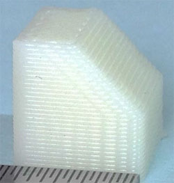 Figure 1: Macrograph of the part (10mm cube with an angled bevel made with 330 μm layers). | A Dimension SST 1200ES Fused Deposition Rapid Prototyping Machine was used to make 10mm cubes with one edge beveled at an angle of 45° (Fig. 1). Layer thicknesses of 250 μm and 330 μm were used. In this fused deposition method, parts were created layer by layer from a thermoplastic extrusion in a semi-liquid state of ABS (two different layer thicknesses were studied). The outer boundary of each layer, which became the surface of the part, was deposited and then the inside was filled. Fused deposition rapid prototyping, also called "fused deposition modeling" (FDM), is an additive manufacturing process (3D printing) commonly used for modeling, prototyping, and production applications. In this case, prototype parts were made using thermoplastic extrusion, in which raw plastic is melted and formed into a continuous profile. |
Surface measurements on the sides, angled bevel face, and top edge were made with an OLYMPUS LEXT OLS4100 laser scanning confocal microscope with the 100x lens. Individual measurements were stitched to cover extended regions. The individual region measurement size was 121 x 121μm, consisting of 1024 x 1024 elevations with an initial sampling interval of 227nm. This initial sampling interval was modified during the subsequent stitching operation.
A slope filter was used in Mountains 7 software (Digital Surf) to remove numerous aberrant heights, or spikes (measurement artifacts that tend to occur in low brightness regions), which were especially prevalent in the narrow regions between the layers. This slope filter removes portions of measurement where slopes are steeper than a threshold selected by the user, in this case 87.5°. This method removes unlikely height measurements without altering the rest of the measurement. The heights where the spikes were removed were replaced using the surrounding average heights, resulting in some smoothing of the measurement where the spikes had been replaced. Despite the smoothing, this process makes measurements more useful by eliminating unrealistic artifacts which would markedly increase the relative lengths and areas.
Measured regions were selected to avoid obvious, large defects in the surfaces, which were cropped from the larger stitched regions and then leveled. This was done with Mountains 7, which was also used to render the measurements into images (Fig. 2).
Using Sfrax fractal analysis software, multi-scale evaluations of the relative lengths of the profiles, and relative areas of surfaces (ASME, 2009), were performed on profiles and surface sections perpendicular to the deposited layers. These selected regions include cross sections of three of the deposited layers (Fig. 2).
Length-scale analysis uses line segments in repeated tiling exercises at different scales to determine profile lengths as a function of scale (ASME, 2009). The length of the line segment represents the scale and remains constant in each individual tiling exercise. Relative lengths are determined at each scale from the ratio of the measured length of the profile to its nominal, or straight-line, length. The relative lengths are calculated over a range of scales from the profile length to the sampling intervals.
Multi-scale evaluation of the relative areas, i.e., area-scale analyses, were performed on selected crests where the layer bulges. Area-scale analyses are similar to length-scale analyses; relative areas are determined, rather than relative lengths. Triangles are used, rather than line segments, to tile areal measurements [z=z(x,y)], rather than profiles [z=z(x)]. (ASME, 2009; ISO 25178, 2012).
Multi-scale discrimination testing was performed on relative areas and their complexities at all the scales in selected regions. (Complexities are the scale-based derivatives determined over decade intervals of the relative lengths or areas. A complexity indicates how the relative lengths or areas change when the scale changes.) The relative areas and their complexities were calculated from a portion of the measurement (192 x 192 μm) of the highest region on one of the deposited layers, as indicated in Figure 2. Form was removed with a second order filter in Mountains 7. These regions were split into four sections (2 x 2) in Sfrax to allow statistical comparisons between the surfaces. An F-test was used to determine the mean square ratio (MSR) which was compared with critical values for determining the level of confidence for discriminating the surfaces based on their relative areas at each of the available scales. (F-tests are used to compare variations within data sets to variations between the data sets to test the significance of these variations.) The MSRs are plotted versus the scale.
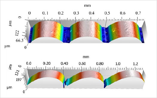
Figure 2 : Rendering of surface measurements from side (above) and angled bevel (below) with 254μm layers.
Results
Renderings of selected portions of surfaces measured from the side and angled bevel of the cube with a layer thickness of 254 μm are shown in Figure 2. A regular pattern corresponding to the layer thickness is evident in Figure 2 (layer thickness is readily detectable from the images). Note that the topographies in the valley regions between the layers have been smoothed by the height replacements after spike filtering.
The values of conventional parameters for the four surfaces are shown in Table 1.
| Parameter | ||||||
| Height (µm) | Hybrid | |||||
| Surface | Sa | St | Sq | Sp | Sdq | Sdr % |
| 254 side | 18.3 | 66 | 20.9 | 25.9 | 0.83 | 21.9 |
| 330 side | 24.3 | 139 | 28.2 | 39.3 | 4.29 | 51.2 |
| 254 angled | 37.1 | 159 | 43.5 | 49.7 | 2.22 | 58.4 |
| 330 angled | 40.1 | 197 | 48.2 | 56.9 | 2.28 | 48.4 |
Table 1 : ISO 25178 height and hybrid parameters (ISO, 2012).
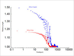 Figure 3 : Relative lengths vs. scales for side and angled bevel surfaces with 254 μm layers. | Plots of the relative lengths versus scale are shown in Figure3 for profiles in the longitudinal direction, i.e., perpendicular to the layers, from the side and angled bevel surfaces shown in Figure 2. Three different regions of scale can be delineated by multi-scale consideration of the relative lengths. At the large scales, above about 250 μm and 350 μm, for the side and angled surfaces respectively, the relative lengths vary regularly and remain close to one. Between these larger scales and a scale of about 30μm for both surfaces, there is a transition region where the relative lengths tend to increase markedly and irregularly. At scales below about 30 μm, the relative lengths continue to increase, although at a lower rate with respect to decreasing scale, until the sampling intervals, 300 to 400nm, are reached. |
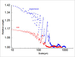 Figure 4 : Larger scale details of the relative lengths vs. scales for side and angled bevel surfaces with 254 μm layers. | Details of the two crossovers between the three regions for relative length are shown in Figure 4. At the largest scales the relative lengths increase slightly, and then return to values close to one again. This happens two times before increasing definitively to larger values at all the finer scales. The finest scale at which the relative length approaches one, before increasing definitively at the finer scales, can be designated as a kind of SRC (Brown, 2000; ASME, 2009; Brown et al., 1996). SRC values are plotted in Figure 5. At the intermediate scales the relative length's irregularity appears to be quasiperiodic, in a series of waves. ("Quasi-periodic" meaning having some similarity to a periodic function but not meeting that function's strict definition.) |
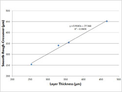 Figure 5 : Smooth-rough crossovers vs. layer thickness and modified thickness for the bevels. | The SRC can be seen to increase linearly with the modified layer thickness (Fig. 5). In Figure 5 the layer thickness on the angled surfaces is modified by multiplying by the square root of two [1/sin(45°)], which is intended to account for the angle of the bevel. The layer thickness and the SRC are shown to be strongly correlated. The regression coefficient (R²) is greater than 0.99, the slope is about 0.9, and the intercept is less than ten percent of the mean value of the SRCs. The height parameters in Table 1 would all increase monotonically, as well, when plotted as in Figure 5. This similarity in trends with the SRC is consistent with the premise that these height parameters are most sensitive to some of the larger scales in the measurements, like the SRC. The hybrid parameters are most sensitive to the finest scales, and do not show similar increases with the modified layer thicknesses. |
The length-scale complexities are compared between the side and the bevel for all of the available scales shown in Figure 6 for the 254 μm and 330 μm layers, respectively. In both cases the angled surfaces tend to have greater complexities than the sides. There is a marked decrease in the complexity in all cases at the finer scales. There is no consistent evidence, however, of any tendency toward a common complexity at the finest scales.
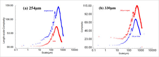
Figure 6: Length-scale complexity vs. scale for the 254 μm layer (left) and 330 μm layer (right).
Rendering of surfaces used for the area-scale analyses, taken from crests of the layer bulges, are shown in Figure. 7. The relative areas, results of the areal multi-scale analyses from the selected crest regions, are shown versus areal scales in Figure 8. The largest linear scale in these analyses is about 30 μm, well below the SRC for relative lengths. The linear scale is half the square root of the triangular areal scale. For all surfaces, with the form removed, the relative areas tend toward one at the largest scales. In these regions, formed removed, the SRCs are about 100 μm² or 5 μm. There appears to be no relation between relative areas and the large-scale processes, i.e., layer thickness and bevel.
Figure 7: Extracted region with form removed from 254 μm crests, side (above) and angled bevel (below).
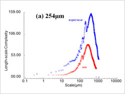 Figure 8: Relative areas vs. scale from the selected crests from the all of the surfaces. | 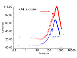 Figure 9: Area-scale complexities shown versus scale for the selected regions. All the surfaces have maximum complexities between 0.4 and 20 μm². |
Figure 10: Multi-scale discrimination from area-scale complexity vs. scale from selected crests from the sides (above) and bevels (below) of 254 and 330 μm layers. | The results of multi-scale discrimination testing using F-tests on the complexities at each scale are shown in Figure 10. The mean square ratio (MSR) is plotted versus scale, and the critical MSR for 99.9% is indicated. In both comparisons, as indicated by the MSR, the ability to discriminate is consistently strong below scales of about 20 μm², strongest at about 10 μm², then diminishes at the finer scales. The ability to discriminate the sides is greater than it is for the angled bevel surfaces as indicated by the MSR values (Fig. 10). |
Acknowledgements
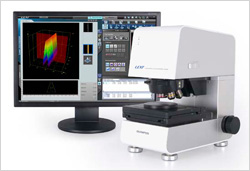 Olympus LEXT OLS4100 Laser Scanning Confocal Microscope | The authors gratefully acknowledge the support of Olympus for the use of the LEXT OLS4100 laser scanning confocal microscope and Digital Surf for Mountains 7 software. Surfract, which supplied the Sfrax software, is owned by co-author Dr. Christopher Brown. |
Conclusion
Multi-scale analysis of the roughness of fused deposition parts is effective at identifying different natures of the topographies at different scales. Integer multiples of the layer thickness correspond to relative minimums in length-scale analyses. At scales just below the layer thickness there is a high degree of complexity in the surface topography. At the finest scales, from hundreds of nanometers to tens of micrometers, the complexity of the surfaces is distinctly less complex than at scales from tens of micrometers to just below the layer thickness.
The topographies at the finest scales retained individuality with respect to the process variables. It is not clear why they should not be more similar. The finest scales were removed from the scale of the layer thickness by three orders of magnitude. It could be supposed that the formation of the roughness at these scales should be similar, regardless of the layer thickness. The hybrid parameters, which have been found to be similar to the relative areas at the finest scales (Berglund et al., 2010), do not rank with the modified layer thickness.
Roughness could be reduced by decreasing the layer thickness. The remaining roughness, shown in Figure 7, is apparently due to other aspects of the process, and might not be eliminated by reducing the layer thickness.
The strong correlations between layer thickness and SRC are similar to those that have been found with feed in turning and SRC (Brown et al., 1996). There is also individuality of the topographies at scales below the feed in turning and below the layer thickness in fused deposition. In both cases, turning and fused deposition, the topography at the scales of what might be called the dominate process variable, feed per revolution and layer thickness, are regular. At finer scales the topographies become chaotic.
The quasi-periodic variation of the relative lengths at and just above and below the scales of the layer thickness is due to the interaction of the tiling algorithm with the larger scale regularity of the layered topography. There is distinct aliasing (distortion) at even multiples of the layer thickness. At those length scales, the tiling algorithm is blind to the topographic variations and the relative lengths tend toward one. At scales just below the layer thickness, the tiling algorithm is interacting in quasi-regular intervals at the scales of different fractions of the layer thickness.
The lack of evidence of a correlation at the finer scales with the dominant process variables could be a function of the small sample size used here. If there were to be some correlation, then the layer thickness could be influencing the formation of the topography at the fine scales. This and the topographic formation mechanisms at the fine scales are beyond the scope of this case study.
Primary conclusions resulting from this case study can be summarized as such:
1. Multi-scale analyses using length-scale and area-scale tilings are able to distinguish regions in scale with distinctly different natures.
2. The relative lengths at scales comparable to the layer thickness and greater show a high degree of regularity. The period depends on the layer thickness and surface orientation.
2.1. The layer thickness appears to be closely related to the scale of the smooth-rough crossover on the length-scale plot.
2.2. The smooth-rough crossover calculated from measurements of the angled bevel region is close to the layer thickness times the sine of 45°.
3. The area-scale complexities of crests of the layer bulges differ significantly between the parts at scales below about 20 μm².
References
Brown C A. Issues in modeling machined surface textures. Machining Science and Technology 2000; 4/3: 539-546.
Ahn D, Kim H, Lee S. Surface roughness prediction using measured data and interpolation in layered manufacturing. Journal of Materials Processing Tech. 2009; 209/2: 664- 671.
Kechagias J. An experimental investigation of the surface roughness of parts produced by LOM process. Rapid Prototyping Journal. 2007; 13/1: 17-22.
ASME B46.1. Surface texture: waviness, roughness and lay. New York: ASME; 2009.
ISO 25178-2, 2012. Geometrical product specifications (GPS) – Surface texture: Areal – Part 2: Terms, definitions and surface texture parameters.
Brown C A, Johnsen W A, Butland R M. Scale-sensitive fractal analysis of turned surfaces. CIRP Annals. 1996; 45/1: 515-518.
Berglund J, Brown C A, Rosen B-G, Bay N. Milled Die Steel Surface Roughness Correlation with Steel Sheet Friction, CIRP Annals. 2010. 59/1: 577-580.