Use of the Total Focusing Method with the Envelope Feature
Nicolas Badeau1 Guillaume Painchaud-April1 Alain Le Duff1
1Olympus NDT Canada
3415 Rue Pierre-Ardouin
Quebec QC, G1P 0B3
Summary
This paper presents how to compute the envelope of a total focusing method (TFM) image and the benefits of using this TFM envelope as part of a code-compliant solution. The TFM envelope is obtained by computing the norm of two different TFM images, namely, a first TFM image computed using the standard acquired full matrix capture (FMC), and a second TFM image computed using the Hilbert transformed FMC. The resulting TFM envelope image provides a better ground for the amplitude-based sizing method as it is more robust to amplitude variation compared with a standard oscillatory TFM image at an identical grid resolution. Therefore, with respect to the standard oscillatory TFM, a coarser grid resolution can be set for the TFM envelope, consequently reducing the total amount of computation effort and ultimately increasing the resulting acquisition rate.
Introduction
The total focusing method (TFM) is a recently accepted technique for nondestructive evaluation of material and structure. Certain standards and codes now include a section on full matrix capture (FMC) and the TFM for nondestructive testing (NDT) [1], [2].
Some NDT devices, such as the OmniScan™ X3 flaw detector, enable real-time TFM imaging. The TFM approach using FMC is summarized in the following section, but the basic premise is that the TFM is based on the summation of a multitude of elementary A-scan amplitude values. The TFM images are oscillatory because of the acoustic wave origins of the elementary A-scans. On the other hand, the characterization schemes found in NDT applications are essentially amplitude-based techniques for which the oscillatory behavior can be seen as a superfluous acoustic artifact. A common practice used to adapt the oscillatory behavior to the characterization schemes is to rectify the amplitude, so the image appears with strictly positive values. While this approach may help ease the interpretation of the image with respect to its fully oscillating counterpart, this paper will show how using the signal envelope may further improve the characterization effort and actually increase the acquisition rate with respect to the standard oscillatory TFM image.
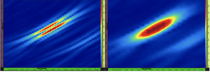
Figure 1—On the left: example of a TFM image of a side-drilled hole (SDH) with strictly positive amplitude values and signal oscillation (i.e. standard TFM). The grid resolution is 0.08 mm (λ / 8.1) and the maximum amplitude is 108.7%. On the right: TFM envelope of the exact same SDH. The grid resolution is 0.16 mm (λ / 4.0) and the maximum amplitude is 122.6%.
There are several disadvantages of using such an oscillatory TFM image. First, the TFM grid resolution—i.e., the distance between two pixels in the frame—must be approximately λ / 8 to be code compliant [1]–[3]. In this article, λ is the wavelength associated with the probe’s central frequency and acoustic velocity in the part. A small grid resolution implies a large computational effort, immediately resulting in a lower acquisition rate. The robustness associated with amplitude-based flaw sizing methods is also impacted by the oscillatory TFM. Indeed, the maximum amplitude of a measured echo is strongly dependent on the phase offset of the acquired signal.
All these issues can be solved using the TFM envelope since it removes the signal oscillations in the image and enables a more robust maximum amplitude measurement (see Figure 1). The acquisition productivity benefits from the use of the TFM envelope as it requires a reduced grid resolution—i.e., larger spacing between two adjacent pixels—for the same amplitude robustness compared with standard TFM. For instance, a grid resolution of approximately λ / 4 is sufficient with the TFM envelope to have the same amplitude fidelity (2 dB) as the standard oscillatory TFM with a resolution of λ / 8 [3].
The goal of this paper is to inform the NDT specialist of the benefits of using the TFM envelope. We first present a recap of the FMC-TFM approach followed by a short presentation of the concepts surrounding the computation of the TFM envelope. Lastly, we present the benefits of using the TFM envelope as part of a code-compliant solution in comparison with standard oscillatory-type TFM images.
Summary of the FMC-TFM Approach
The hallmark of ultrasonic phased array is the capacity to focus at any desired position in a part being inspected. The phased array focusing approach uses delays, both in transmission and reception, to synchronize the time of flights of short, pulsed signals at the position of interest. At the focal zone in the specimen, the overall width of the generated acoustic beam becomes small, and the corresponding detection resolution increases dramatically [4]–[12].
The TFM is a natural extension of this capacity; the TFM produces a focused beam through phased array focalization and steering at every position over a region of interest inside a part being inspected, and only the set of highly resolved focalized data points are presented to the operator [13]–[16]. Often, the region of interest consists of a uniform Cartesian grid of all the requested focalization targets. Obviously, achieving this focalization at each grid position using the conventional physical beamforming approach would prove exceedingly time consuming because of the physical acoustic propagation time required to reach every position of interest.
Since the typical ultrasonic acoustic waves for NDT applications are linear, the physical beamforming resulting from the superposition of actual acoustic fields for all contributing elements of a given aperture can be emulated by a post-acquisition process based on the full matrix capture (FMC) data set. Retrieving the FMC data set requires recording the signal from all elements composing the receiving aperture while an acoustic emission is produced by every individual element comprising the transmission aperture. As such, the FMC data set is formed by the multitude of elementary A-scans for all combinations of transmitting and receiving elements.
As with conventional focused phased array, obtaining the focalized amplitude from a given focalization position requires the following:
- The computation of the time of flight needed for the acoustic propagation to reach the focal position matching a selected grid position of interest and back to the receiving element, for all pairs of transmission and reception elements of the aperture
- The selection of the amplitude data point corresponding to the appropriate complete transmission-reception time of flight for all pairs of transmission and reception elements of the aperture
- The summation of all selected amplitude data points over all contributing elements of the transmission and reception apertures
- The placement of the resulting summed amplitude at the initially selected grid position
Repeating these steps for all grid positions over the region of interest produces an amplitude map for which all amplitude values correspond to a focalized beam, both in transmission and reception. This method of using the FMC data to produce a map of amplitude focalized at each position over the region of interest (i.e., the TFM zone) is referred to as the FMC-TFM approach.
How the TFM Envelope Is Computed
This section describes how the TFM envelope is computed using the same elementary A-scans (FMC) acquired for the standard TFM. It should be noted that the envelope has a physical manifestation and is not a mere image smoothing algorithm. The envelope on the TFM image has its roots in its constituting individual A-scans. First, to schematically illustrate its behavior, the envelope concept is presented using a Gaussian pulse time series. The process is also applied to an empirical A-scan and on a complete TFM frame.
The signal a(t) corresponds to the acquired signal—i.e., the equivalent of an elementary A-scan acquired through FMC—and is, in fact, the real part of a complex analytical signal z(t), which can be written as
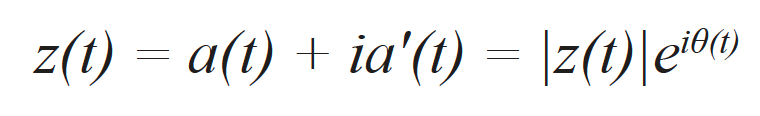
where a’(t) corresponds to the imaginary part of the analytical signal, and θ(t) is the instantaneous phase of the signal. The imaginary part is effectively computed using the Hilbert transform [17]. The signal envelope corresponds to the norm of the analytical signal, which can be written as
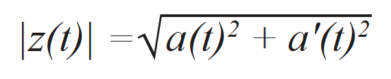
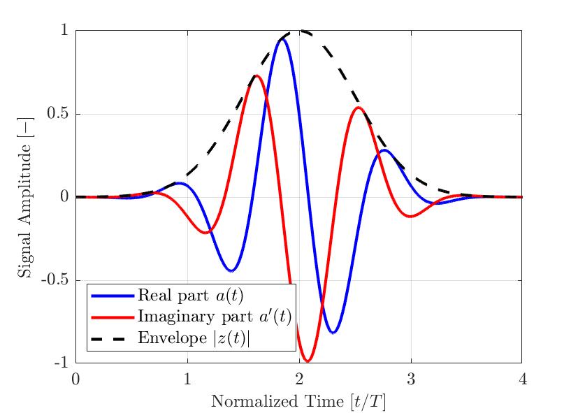
Figure 2— A typical Gaussian-modulated pulse for NDT applications. The real and imaginary parts and computed envelope are shown. The time axis is normalized with the selected central frequency period of the pulse.
Figure 2 shows an example of a simple Gaussian-modulated pulse a(t). The real signal a(t) is in blue, its Hilbert transformed imaginary part a’(t) is in red, and the resulting envelope |z(t)| is a dashed line. As seen in the equation above, the signal envelope |z(t)| is not affected by the instantaneous phase θ(t) of the signal. Hence, signals with different phase offsets ϕ can have the same envelope. Figure 3 illustrates several Gaussian-modulated pulses with different phase offsets ϕ and their resulting envelope. Therefore, the measured maximum amplitude of the signal is more robust when using the signal envelope than the absolute value of the real component of the analytical signal.
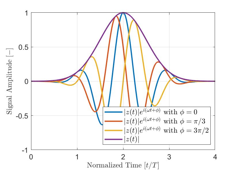
Figure 3—Typical Gaussian-modulated pulses (|z(t)|ei(ωt+ϕ)) with different phase offsets ϕ. The envelope |z(t)| of the signals is clearly independent of the instantaneous phase of the analytical signal.
The same process can be used to obtain the envelope of an empirical A-scan. Figure 4 shows a typical elementary A-scan acquired through FMC, while Figure 5 shows the same A-scan (blue) with its Hilbert transform (red) and the computed envelope (dashed line). All signals shown are normalized to the maximum of the amplitude envelope.
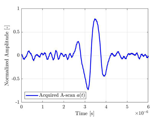 Figure 4—Portion of an acquired elementary A-scan (from an FMC acquisition). | 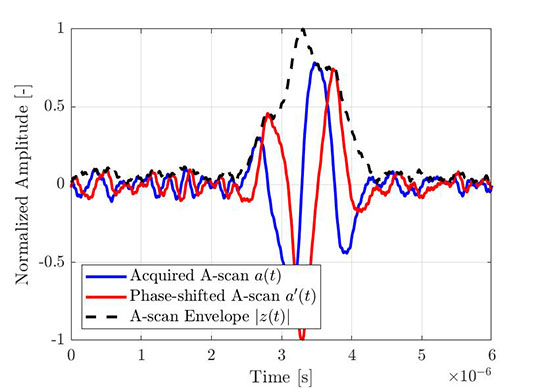 Figure 5—The same elementary A-scan with its Hilbert transform and the computed envelope. |
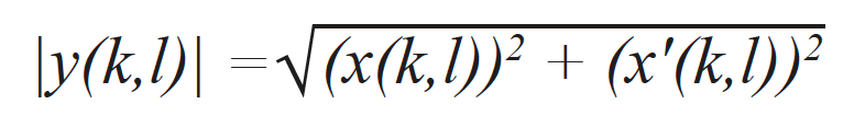
The TFM envelope image—with individual grid point indexes (k,l)—is computed using the analytic signals from all its contributing A-scans [15]. It is, in fact, the result of computing the norm of an analytic TFM image y(k,l) composed of the standard TFM frame x(k,l) computed using the standard FMC acquired data and a TFM frame x'(k,l) computed with the Hilbert transform of the FMC data. The same set of delays is used in both cases. The TFM envelope is then computed using the following expression
A TFM envelope image is, therefore, the result of a combination of two TFM images (see Figure 6): one from the real component of the elementary A-scans and the other from the computed imaginary component of the elementary A-scans. While this process increases the computation burden and reduces the NDT instrument’s acquisition speed, we demonstrate in the next section that the required grid resolution can be reduced significantly without affecting the amplitude fidelity, increasing the acquisition speed to a rate that is higher than when using the standard TFM.
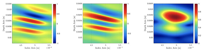
Figure 6—Left: standard TFM frame (not in absolute value). Center: TFM frame computed using the Hilbert transform of the FMC. Right: resulting TFM envelope image.
Advantages of Using the TFM Envelope
In this section, we demonstrate the TFM envelope’s advantages by comparing several TFM frames with different grid resolution ratios, ranging from λ / 9.3 to λ / 4.0, and monitoring various critical inspection metrics. The results were obtained using a 5L32-A31 probe and an SA31-N55S-IHC wedge on a steel block with a 1 mm diameter side-drilled hole (SDH) (see Figure 7). A coupling gel (Sonotech Ultragel II) is used between the wedge and the steel block. Data are acquired using the Olympus OmniScan™ X3 flaw detector. The pulse-echo (T-T) acoustic path is selected, and the zone size is (20 mm × 20 mm). The wavelength associated with the part and acoustic path selected is λ = 0.648 mm. The grid resolution is noted in terms of wavelength fraction.
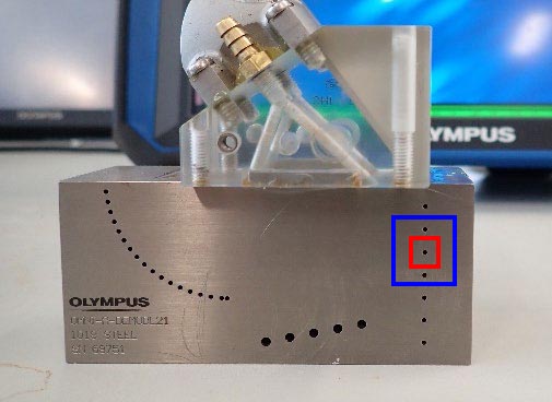
Figure 7—A photo of the setup used to acquire the TFM images in Table 1. The blue rectangle corresponds to the entire region of interest (20 mm × 20 mm) while the red rectangle corresponds to the zoomed region of interest (5 mm × 5 mm) shown in the Table 1 images. We used a 5L32-A31 probe and SA31-N55S-IHC wedge. The steel block has a thickness of 40 mm.
Table 1 shows the resulting TFM images for four different grid resolution values, ranging from λ / 9.3 to λ / 4.0, for both the standard TFM and the TFM envelope. The computed amplitude fidelity value [3] and the resulting acquisition rate are indicated on each of the TFM images.
Grid Resolution | Standard TFM | TFM Envelope |
|---|---|---|
λ / 9.3 | 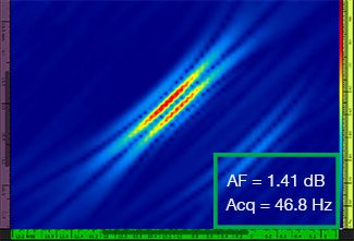 | 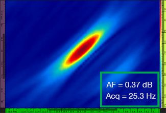 |
λ / 8.1 | 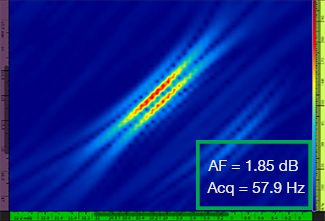 | 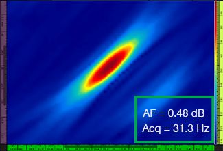 |
λ / 5.9 | 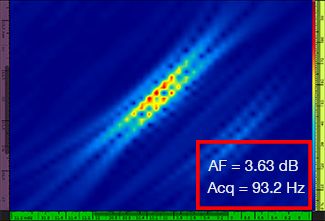 | 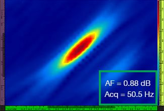 |
λ / 4.0 | 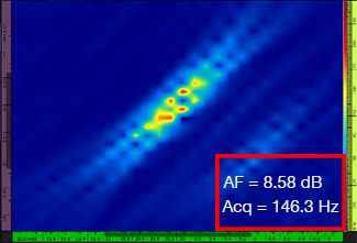 | 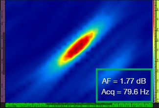 |
Table 1—Comparing the image quality between standard TFM and the TFM envelope at four grid resolution values. The TFM images shown are zoomed in. On the figures, AF means amplitude fidelity and Acq corresponds to the acquisition rate obtained with the specified grid resolution. The red boxes indicate a failure to achieve a code-compliant 2 dB amplitude fidelity value. Note the higher acquisition rate at equivalent AF value.
Newly available codes and standards [1, 2] require the amplitude fidelity value to be 2 dB or less. Hence, only the first two grid resolution values (λ / 9.3, λ / 8.1) are code compliant when using the standard TFM. The TFM envelope enables a coarser grid resolution (λ / 4.0) while maintaining a code-compliant amplitude fidelity. In turn, using the TFM envelope with a coarser grid induces an increase in acquisition speed of approximately 37% with respect to the highest acquisition rate achieved by the code-compliant standard TFM (57.9 Hz at λ / 8.1).
Conclusions
The method to compute the envelope of a TFM image was presented and illustrated using simple examples. We demonstrated that the envelope of a signal is independent of its instantaneous phase and, therefore, provides a more robust basis for amplitude-based sizing techniques (such as the 6 dB drop method). The signal envelope is not merely image smoothing and should not be regarded as a filter, which can engender data losses. The advantages of using the envelope in TFM imaging were demonstrated through comparisons of TFM images, with and without the envelope, for different grid resolution values. Although two TFM images must be computed to obtain the resulting TFM envelope, the processing burden can be reduced significantly by using a coarser grid resolution while remaining code compliant. This is due to the robustness of the envelope with regards to amplitude variation. The result is an image that is more adapted to amplitude sizing yet obtained at a faster pace than the equivalent image processed using standard TFM.
References
[1] ASME Committee, “ASME BPVC.V Article 4 Mandatory Appendix XI Full Matric Capture.” ASME, 2019.
[2] ASME Committee, “ASME BPVC.V Article 4 Nonmandatory Appendix F - Examination of Welds Using Full Matric Capture.” ASME, 2019.
[3] N. Badeau, A. Le Duff, and C.-H. Kwan, “Theoretical Model for Amplitude Fidelity Reading (submitted),” presented at the ASNT Research Symposium, 2020.
[4] A. C. Clay, S.-C. Wooh, L. Azar, and J.-Y. Wang, “Experimental Study of Phased Array Beam Steering Characteristics,” Journal of Nondestructive Evaluation, vol. 18, no. 2, p. 13, 1999.
[5] L. J. Bond, “Fundamentals of Ultrasonic Inspection,” ASM Handbook, vol. 17, no. Nondestructive Evaluation of Material, pp. 155–168, 2018.
[6] S.-J. Song, H. J. Shin, and Y. H. Jang, “Development of an ultra sonic phased array system for nondestructive tests of nuclear power plant components,” Nuclear Engineering and Design, vol. 214, no. 1–2, pp. 151–161, May 2002, doi: 10.1016/S0029-5493(02)00024-9.
[7] S. Mahaut, O. Roy, C. Beroni, and B. Rotter, “Development of phased array techniques to improve characterization of defect located in a component of complex geometry,” Ultrasonics, vol. 40, no. 1–8, pp. 165–169, May 2002, doi: 10.1016/S0041-624X(02)00131-2.
[8] S. C. Mondal, P. D. Wilcox, and B. W. Drinkwater, “Design of Two-Dimensional Ultrasonic Phased Array Transducers,” Journal of Pressure Vessel Technology, vol. 127, no. 3, pp. 336–344, Aug. 2005, doi: 10.1115/1.1991873.
[9] S.-C. Wooh and Y. Shi, “Influence of phased array element size on beam steering behavior,” Ultrasonics, vol. 36, no. 6, pp. 737–749, Apr. 1998, doi: 10.1016/S0041-624X(97)00164-9.
[10] Joon-Hyun Lee and Sang-Woo Choi, “A parametric study of ultrasonic beam profiles for a linear phased array transducer,” IEEE Trans. Ultrason., Ferroelect., Freq. Contr., vol. 47, no. 3, pp. 644–650, May 2000, doi: 10.1109/58.842052.
[11] R. Ahmad, T. Kundu, and D. Placko, “Modeling of phased array transducers,” The Journal of the Acoustical Society of America, vol. 117, no. 4, pp. 1762–1776, Apr. 2005, doi: 10.1121/1.1835506.
[12] B. W. Drinkwater and P. D. Wilcox, “Ultrasonic arrays for non-destructive evaluation: A review,” NDT & E International, vol. 39, no. 7, pp. 525–541, Oct. 2006, doi: 10.1016/j.ndteint.2006.03.006.
[13] P. D. Wilcox, “Exploiting the Full Data Set from Ultrasonic Arrays by Post-Processing,” in AIP Conference Proceedings, Brunswick, Maine (USA), 2006, vol. 820, pp. 845–852, doi: 10.1063/1.2184614.
[14] J. Zhang, B. W. Drinkwater, and P. D. Wilcox, “Effects of array transducer inconsistencies on total focusing method imaging performance,” NDT & E International, vol. 44, no. 4, pp. 361–368, Jul. 2011, doi: 10.1016/j.ndteint.2011.03.001.
[15] C. Holmes, B. W. Drinkwater, and P. D. Wilcox, “Advanced post-processing for scanned ultrasonic arrays: Application to defect detection and classification in non-destructive evaluation,” Ultrasonics, vol. 48, no. 6–7, pp. 636–642, Nov. 2008, doi: 10.1016/j.ultras.2008.07.019.
[16] C. Holmes, B. W. Drinkwater, and P. D. Wilcox, “Post-processing of the full matrix of ultrasonic transmit–receive array data for non-destructive evaluation,” NDT & E International, vol. 38, no. 8, pp. 701–711, Dec. 2005, doi: 10.1016/j.ndteint.2005.04.002.
[17] D. Gabor, “Theory of Communication,” Journal of the Institution of Electrical Engineers, vol. 96, pp. 429–441, 1946.