TFM Acoustic Influence Map
Chi-Hang Kwan
Guillaume Painchaud-April
Benoit Lepage
Paper originally presented at the 2019 ASNT Research Symposium.
ABSTRACT
In this paper, we introduce a newly developed semi-analytical model to predict the total focusing method (TFM) amplitude sensitivity map for both nondirectional and directional flaws. For complicated acoustic paths that involve multiple interface interactions and wave-mode conversions, a knowledge of the Acoustic Influence Map (AIM) enables an inspector to refine the scan plan to maximize the signal-to-noise ratio of the resultant TFM image and increase the probability of flaw detection. The accuracy of this new acoustic model was tested and validated by experiments using test blocks that contain side-drilled holes and flat-bottom holes. Results from the validation experiments show good agreement between the empirical TFM amplitude maps and theoretical AIM. The results also indicate that the model can be used to guide the selection of the optimal TFM inspection mode.
INTRODUCTION
The total focusing method (TFM) is a synthetic aperture beam forming technique that has been under active development in the NDT industry over the past decade [1]. By applying appropriate transmission and reception delays to A-scan data collected in a full matrix capture (FMC) dataset, TFM can electronically focus on every location within an inspection region. Since every point is electronically focused, TFM can provide better resolution compared to conventional phased array ultrasound inspection techniques. In addition, by calculating and applying the time of flights of multiple acoustic modes, multi-mode TFM that can provide additional information about the specimen being inspected [2].
Despite the advantages listed above, TFM also has limitations governed by physical laws. An inspection area may have poor sensitivity due to the effects of interface interaction, beam forming limitations, and propagation path attenuation. Owing to the novelty of TFM, the lack of inspection codes, and the complexity of multi-mode TFM imaging, inspectors are generally unaware of the physical limits of TFM and, therefore, cannot define an optimal scan plan that maximizes the signal-to-noise ratio (SNR) and the probability of detection. Consequently, there is a need to introduce a tool that estimates the acoustic sensitivity map for a given TFM inspection scan plan.
ACOUSTIC REGION OF INFLUENCE
The Acoustic Influence Map (AIM) is a theoretical acoustic amplitude sensitivity map for a given TFM inspection scan plan. In general, the AIM differs for directional and nondirectional flaw scatterers. NDT examples of nondirectional scatterers include slag and porosity in welds, while examples of directional scatterers include lack of fusion in welds and various cracks. The directional scattering response of a flaw is an important parameter that is often neglected in the modeling of phased array transducer systems.
To calculate the AIM, we have developed a semi-analytical, ray-based acoustic model that calculates the two-way pressure response of pulse-echo, self-tandem, and double-skip TFM inspection modes. This acoustic model takes into account the effects of transmission and reflection coefficients, geometric beam spread, and material attenuation. In addition, in our model, we also used the Rayleigh-Sommerfeld integral [3] to model the far-field scattering response for a flat-bottom hole (FBH). The FBH scattering response is used to simulate directional flaws.
VALIDATION EXPERIMENTSTo examine the acoustic model’s accuracy, we conducted validation experiments to compare experimentally obtained TFM amplitude maps with a theoretically calculated TFM AIM. Results obtained from two validation experiments are presented in this section. The first validation experiment was conducted on a test block that contains small-diameter side-drilled holes (SDHs), which simulate the scattering response of nondirectional flaw scatterers. The second validation experiment was conducted on a test block that contains FBHs, which simulate the scattering response of directional flaws. For the results presented in this paper, the x-axis is defined positive to the right of the first transducer element, and the z-axis is defined positive below the surface of the test sample. A schematic diagram of this coordinate system is shown in Figure 1. | 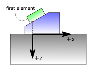 Figure 1: Coordinate system used in this paper. |
Side-Drilled Hole Validation
The SDH validation experiment was conducted on a NAVSHIPS metric 1018 steel test block that contains six 1.2 mm (0.05 in.) diameter SDHs at depths from 6.25 mm (0.25 in.) to 37.5 mm (1.5 in.) in 6.25 mm increments. By turning over the test block, it is possible to examine SDHs at depths from 6.25 mm (0.25 in.) to 68.75 mm (2.7 in.). For this experiment, we used a 32-element 5L32-A31 probe with a center frequency of 5 MHz and an element pitch of 0.6 mm. The probe was coupled to a 36.1º SA31-N55S-IHC Rexolite wedge. A schematic drawing of the experimental setup is shown in Figure 2.
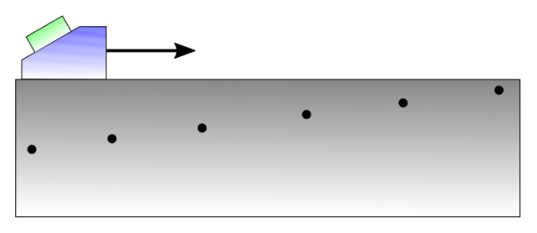
Figure 2: Schematic diagram of the SDH validation experiment. Note that only the top scan orientation is shown.
By translating the probe along the surface of the test block, we obtained scattering echoes from the SDHs at different positions relative to the probe. FMC datasets were gathered at each scan position for post-processing to generate empirical TFM amplitude maps. A description of the post-processing algorithm is described in the following subsection.
Generating the Empirical TFM Amplitude Map
The main steps for generating the empirical TFM amplitude map are:
- For a given flaw at a fixed scan position, use a depth (z-direction) gate to obtain an amplitude line along the width of the amplitude map.
- Repeat step 1 for different scan positions to obtain a composite amplitude line for a given flaw.
- Repeat steps 1 and 2 for all other flaws to obtain composite amplitude lines at different z-positions.
- Interpolate the composite amplitude lines in the z-direction to obtain the final TFM amplitude map.
Step 1 is illustrated in Figure 3. Figure 3 shows that we first form a TFM strip along the width of the amplitude map at depths specified by the z-gate. The position of the z-gate is chosen based on the known depth of the flaw. At every x-position along the TFM strip, the maximum amplitude is taken along the z-direction to obtain the amplitude line shown at the bottom of Figure 3.
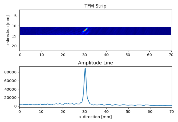
Figure 3: Procedure to obtain an amplitude line for a given flaw at one scan position.
To form the composite amplitude line for a given flaw, we compare all amplitude lines obtained at different scan positions and record the maximum amplitude values. This procedure is illustrated in Figure 4.
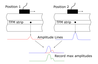
Figure 4: The procedure to form composite amplitude lines at different scan positions.
After forming the composite amplitude line for a given flaw, the process is repeated for all flaws at different depths. Figure 5 shows the pulse-echo TT mode composite amplitude lines obtained for the SDHs present in the NAVSHIPS test block (both top and bottom orientations). In Figure 5 and all other experimental TFM-derived figures presented in this paper, the amplitudes of the TFM images are not normalized. Since a 12-bit digitizer is used in the acquisition electronics and the probe contains 32 elements, the theoretical maximum amplitude in the TFM image is 2097152 (212 ÷ 2 × 32 × 32).
Note that the composite amplitude lines for SDHs at depths of 6.25 mm (0.25 in.), 62.5 mm (2.5 in.), and 68.75 mm (2.7 in.) were not included in Figure 5. Due to the proximity of these SDHs to the lateral limits of the test block, it was not possible to obtain complete composite amplitude lines along the entire width of the amplitude map.
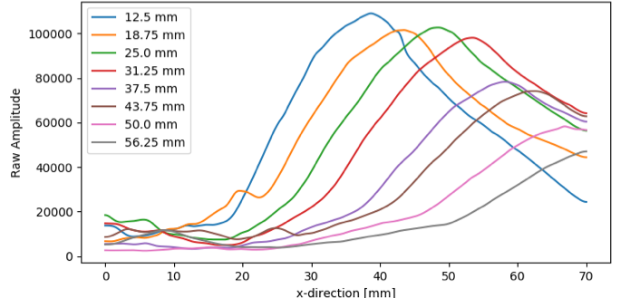
Figure 5: The composite amplitude lines of SDHs present in the NAVSHIPS test block.
Comparing Empirical TFM Amplitude Maps with AIM
By performing z-direction interpolation on the composite amplitude lines shown in Figure 5, we obtained the empirical TFM amplitude map shown in Figure 6 (a).
Figure 6 (a) shows that this TFM scan plan has poor sensitivity both at low (30º) and high (>70º) steering angles. The poor sensitivity at low steering angles is caused by small transmission coefficient values from the Rexolite wedge to the steel test block [4]. In contrast, the poor sensitivity at high steering angles is due to poor focusing caused by large effective F-numbers [5]. These findings are consistent with the recommended steering angle guidelines for conventional phased array angled inspections [6].
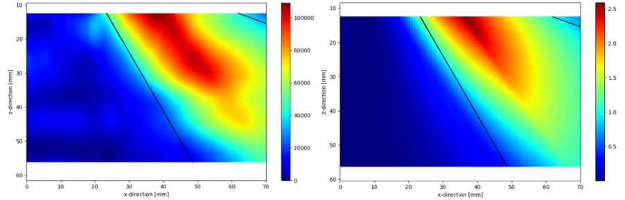
Figure 6: (a) Empirical SDH amplitude map and (b) theoretical SDH AIM for pulse-echo TT mode. 30º and 70º steering angle guidelines (from the midpoint of the active aperture) were added. The corresponding theoretical SDH AIM is shown in Figure 6 (b).
Comparing figures 6 (a) and (b), it is evident that the acoustic model can accurately predict the area within the scan plan that has the optimal sensitivity. The discrepancies between the two figures can be attributed to small variations in coupling pressure as the probe is translated along the test block’s surface. Note that the amplitude of the theoretical AIM is in arbitrary units because it is extremely difficult to model the exact magnitude of the received voltage signals from the acquisition system. However, since consistent arbitrary units are used for different AIMs, it is still possible to compare the TFM acoustic sensitivities of different scan plans and different acoustic modes.
Flat-Bottom Hole Validation
To test the accuracy of the acoustic model for predicting the amplitude sensitivity for directional flaws, we conducted validation experiments on a custom-machined test block. The test block has a thickness of 20 mm (0.8 in.) and contains FBHs that were drilled to match the profile of a typical J-bevel weld. For this study, we use the 5 FBHs whose bottom surface normal vectors are oriented 3º below horizontal. A photograph of the test block with indications of the scan axes is shown in Figure 7.
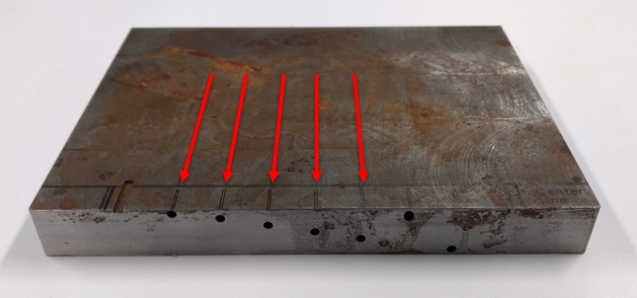
Figure 7: Custom-machined FBH test block showing the scan axes.
For this experiment, we used a 32-element 5L32-A32 probe with a center frequency of 5 MHz and an element pitch of 1 mm. The probe was coupled to a 36.1º SA32-N55S-IHC Rexolite wedge. Since the orientations of the bottom surfaces of the FBHs are near vertical, the acquired FMC datasets were processed in self-tandem (single skip) modes. A schematic diagram of the scan plan is shown in Figure 8.
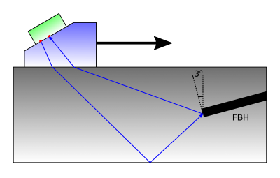
Figure 8: A schematic diagram of the validation experiment showing the self-tandem TFM mode.
Comparing Empirical TFM Amplitude Maps with AIM
The empirical FBH amplitude map and the theoretical FBH AIM for self-tandem TTT mode are respectively shown in Figure 9 (a) and (b). Comparing the two plots, it is evident that the acoustic model provided an accurate estimate of the relative acoustic sensitivity within the scan region. Figure 9 suggests that self-tandem TTT is better suited for detecting vertical flaws located near the bottom of the test sample.
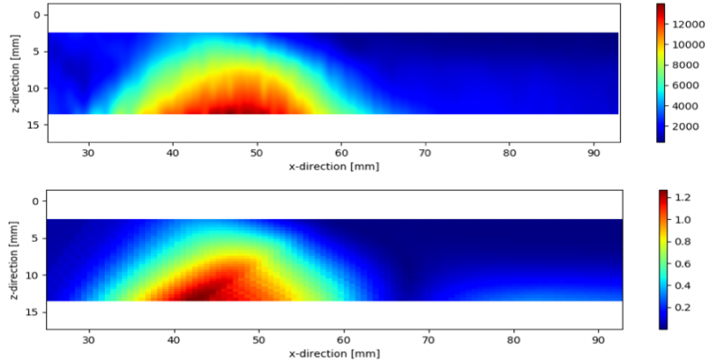
Figure 9: (a) Empirical FBH amplitude map and (b) theoretical FBH AIM for self-tandem TTT mode.
The empirical FBH amplitude map and the theoretical FBH AIM for self-tandem TLT mode are respectively shown in Figure 10 (a) and (b). Once again, it is evident that the acoustic model provided an accurate estimate of the relative acoustic sensitivity within the scan region. The oscillations of the empirical amplitude map from x = 25 mm (1 in.) to x = 40 mm (1.6 in.) are caused by interference from other acoustic modes that have similar travel times.
In addition, comparing Figure 9 with Figure 10, we see that the ratios of maximal amplitudes between the two self-tandem modes are approximately 3.3 (13800/4200) for the empirical amplitude maps and approximately 3.4 (1.23/0.36) for the theoretical AIM. The similarity of amplitude ratios suggests that the acoustic model can also be used to predict the relative acoustic sensitivity across different TFM imaging modes.
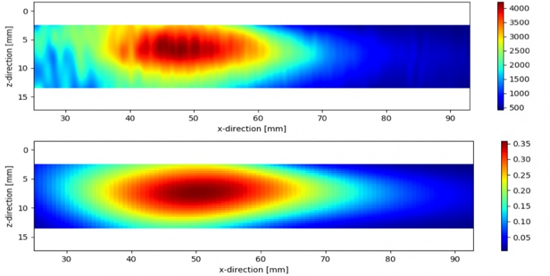
Figure 10: (a) Empirical FBH amplitude map and (b) theoretical FBH AIM for self-tandem TLT mode.
EXAMPLE APPLICATION
To further demonstrate the utility of the acoustic model, we present an example of a real-world application where the theoretical AIM is used to guide our selection of the TFM inspection mode. For this example, we inspected a V-bevel weld sample with a known lack of fusion defect. The weld angle is approximately 35º, and we used the same 5L32-A32 probe and SA32-N55S-IHC wedge that was used for the FBH validation experiment. A schematic diagram of the experimental setup is shown in Figure 11.
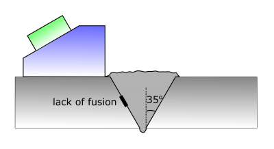
Figure 11: Schematic diagram for lack of fusion inspection.
In the theoretical model, the lack of fusion defect is simulated by a 5 mm (0.2 in.) diameter FBH defect that has a bottom surface oriented at 35º away from the vertical. The corresponding theoretical AIM for self-tandem TLT mode and double-skip TTTT mode are shown in Figure 12.
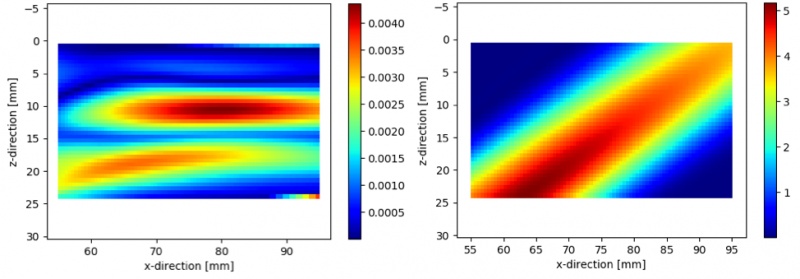
Figure 12: Theoretical AIM for a lack of fusion inspection plan in (a) self-tandem TLT mode and (b) double-skip TTTT mode.
Figure 12 shows that the TLT mode AIM is more irregular compared to the double-skip mode AIM. Consequently, it would be more difficult to obtain a robust assessment of the size of the lack of fusion defect using TLT mode. In addition, the expected amplitude from the TLT mode is 3 orders of magnitude lower than the double-skip mode. Using these theoretical AIMs, we predict that the double-skip TTTT mode is the preferred TFM imaging mode. The corresponding experimental TFM images are displayed in Figure 13.
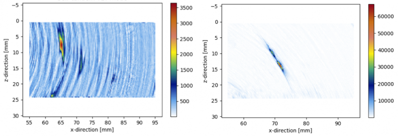
Figure 13: TFM images of a lack of fusion defect in (a) self-tandem TLT mode and (b) double-skip TTTT mode.
Figure 13 demonstrates that the double-skip TFM image has good a good SNR and provides a clear assessment of the size of the lack of fusion defect. In contrast, the self-tandem TFM image has a poor SNR and contains isolated echoes that are difficult to interpret. The isolated echoes are likely the diffracted echoes from the sharp tips of the lack of fusion defect. Nevertheless, the dimension and type of defect are difficult to assess in self-tandem TLT mode.
The poor SNR of the self-tandem TLT mode TFM image corroborates with the low amplitude shown in the theoretical AIM in Figure 12 (a). However, it should be noted that the ratio of echo amplitudes for the two modes in Figure 13 is lower than the amplitude ratio predicted by the theoretical AIM in Figure 12. Since the geometry of the lack of fusion defect is different from the FBH model used to simulate the flaw, the amplitudes of the diffracted echoes from the sharp tips of the lack of fusion defect might be underestimated in the theoretical model.
CONCLUSIONS
We have demonstrated an acoustic model that can accurately predict the TFM amplitude map for both nondirectional and directional defects. For a given inspection mode, the model can be used to adjust the scan plan (aperture, scan frequency, probe location, etc...) to optimize the SNR and the probability of detection. Since the model provides a comparison of relative amplitude across different acoustic modes, it can also be used to select the optimal TFM reconstruction mode. In the future, we plan to extend the model to more complex geometries and include more flaw scattering models to increase the utility of the model.
REFERENCES
[1] C. Holmes, B. W. Drinkwater, and P. D. Wilcox, “Post-processing of the full matrix of ultrasonic transmit–receive array data for non-destructive evaluation,” NDT E Int., vol. 38, no. 8, pp. 701–711, Dec. 2005.
[2] K. Sy, P. Bredif, E. Iakovleva, O. Roy, and D. Lesselier, “Development of methods for the analysis of multi-mode TFM images,” J. Phys. Conf. Ser., vol. 1017, p. 012005, May 2018.
[3] L. W. S. Jr, Fundamentals of Ultrasonic Nondestructive Evaluation: A Modeling Approach, 2nd ed. Springer International Publishing, 2016.
[4] Foundations of Biomedical Ultrasound. Oxford, New York: Oxford University Press, 2006.
[5] S. I. Nikolov, J. Kortbek, and J. A. Jensen, “Practical applications of synthetic aperture imaging,” in 2010 IEEE International Ultrasonics Symposium, San Diego, CA, 2010, pp. 350–358.
[6] E. A. Ginzel and D. Johnson, “Phased-Array Resolution Assessment Techniques,” p. 13.