Authors: Nicolas Badeau, Guillaume Painchaud-April, and Chi-Hang Kwan
Summary
The total focusing method (TFM) inspection technique is now included in codes and standards governing nondestructive testing (NDT), such as ASME Section V. One important parameter specified in these codes for TFM scan planning is the amplitude fidelity. It is defined as the amplitude variation obtained for a specified reflector, owing to the finite resolution of the imaging grid. The typical allowable amplitude fidelity threshold in these codes is a maximum of 2 dB. While experimental methods are suggested by the codes to measure the amplitude fidelity of a given setup, a simple and conservative analytical method is proposed in this paper. The use of the TFM envelope is also considered in the amplitude fidelity estimation since it enables a less dense TFM grid to be used without causing the amplitude fidelity value to exceed the established tolerance. For standard TFM imaging, empirical results showed that a grid resolution of about λ0/10 is required to obtain an amplitude fidelity of less than 2 dB. For TFM imaging with the envelope, the empirical results showed the need for grid resolution of λ0/3.3 to be code compliant.
Introduction
The total focusing method (TFM) is a newly accepted technique for nondestructive testing (NDT) of components. Standards and codes, such as ASME V [1], have integrated full matrix capture (FMC) and TFM as an additional phased array ultrasonic inspection technique. While FMC/TFM is relatively new in the NDT industry, it has been used for some time in medical applications as the gold-standard for medical ultrasonic imaging [2–4]. Indeed, most medical ultrasonic imaging techniques are usually benchmarked and compared with TFM imaging.
While several techniques similar to FMC/TFM exist (e.g., VTFM [5], IWEX [6], SAFT [7]), the most common algorithm used is delay-and-sum processing [2–4,8,9]. The FMC/TFM technique consists of an acquisition scheme (FMC), which relies on acquiring the signal from all combinations of transmitter and receiver elements, and a summation scheme (TFM), which computes the result of the focalized ultrasonic beam at multiple locations in a region of interest. The TFM region of interest is often meshed over a Cartesian grid, and individual grid intersections at which the acoustic focalization is applied are referred to as pixels. The focalization method is similar to standard phased array ultrasonic imaging, except that the beams are formed in post-processing using the data stored in the FMC matrix of data. The post-acquisition delay-and-sum process assumes the linearity of the underlying acoustic waves found in typical NDT applications.
The FMC/TFM technique can be seen as a natural extension of the conventional phased array technique. However, new setup parameters must be considered because of the differences in data representation compared with conventional phased array ultrasonic testing (PAUT). One such concept is the amplitude fidelity (AF) of a TFM grid. AF is defined as the maximum amplitude variation of an indication caused by the TFM grid resolution {Δx,Δz}. The use of a uniform Cartesian grid, i.e. (Δx=Δz), is considered for the remainder of this study. The amplitude fidelity can be formally expressed as
![(Eq.1) AF(Δx)≡-20 log〖(A_(sampled max) (Δx))/A_(true max) 〗 [dB]](https://static3.olympus-ims.com/data/Image/white-papers/amplitudeFidelity/wpaper_amplitudeFidelity_01.jpg?rev=17FA)
where Asampled max is the measured maximum amplitude of a feature of interest based on a finite grid sampling, and Atrue max is the maximum of the same feature of interest based on an infinite grid resolution. The limit at which the grid size becomes zero over the two axes for Asampled max (Δx) defines Atrue max, and the corresponding amplitude fidelity becomes  AF(Δx)=0. Equation 1 provides a formal definition to compute the amplitude fidelity with respect to grid resolution. In practice, however, the true maximumm Atrue max of the underlying signal can only be estimated by oversampling of the TFM amplitude image, and interpolation,
![(Eq.2) (AF) ̂(Δx)=-20 log〖(A_(sampled max) (Δx))/A ̂_(true max) 〗 [dB]](https://static5.olympus-ims.com/data/Image/white-papers/amplitudeFidelity/wpaper_amplitudeFidelity_02.jpg?rev=17FA)
where ![]() true max is an estimator of Atrue max.
true max is an estimator of Atrue max.
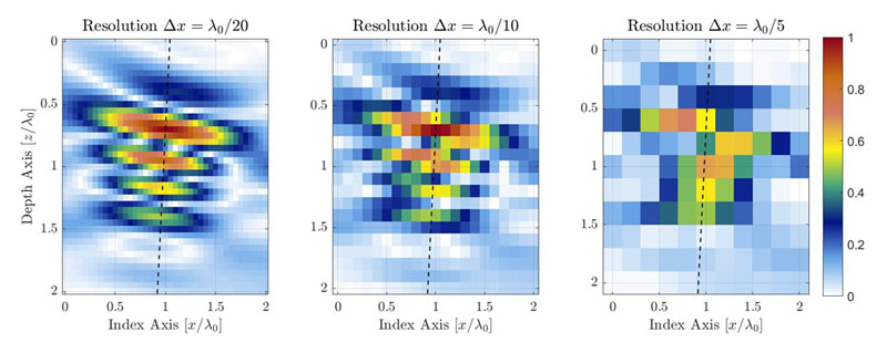
Figure 1. Illustration of the TFM image quality degradation caused by decreasing TFM grid resolution. The dashed lines represent the principal axis of acoustic propagation.
For an identical zone of interest, a coarser grid resolution will have a lower pixel count. Figure 1 shows typical TFM images of the same side-drilled hole (SDH) for different grid resolution values. The grid resolution is defined as a fraction of the probe central frequency wavelength λ0= c/f0, where is the acoustic velocity in the part, and f0 is the probe central frequency.
Standards and codes now include a requirement for the amplitude fidelity to be at a maximum of 2 dB [1,10]. This requirement arises from the applicative compromise between sufficient image quality to ensure proper NDT analysis, and inspection productivity, which is deeply impacted by the density of the TFM grid over a given region of interest. Note that the balance between TFM image quality and inspection productivity is especially critical for autonomous portable devices that do not have access to a large amount of processing power. This issue is expected to disappear over time as embedded hardware improves in power efficiency, and remote computation becomes widely available.
While some empirical methods have been proposed [10–12], they usually require extensive computation, and the results obtained are not representative of the true amplitude caused by the grid resolution, which is an issue that will be explained in the following section. This paper presents a method to accurately estimate the amplitude fidelity of a TFM setup to help the NDT technician perform a code compliant and productive TFM inspection.
The paper is divided as follows. First, a comprehensive explanation of the problem faced by NDT technicians is given. Then a method to empirically measure the amplitude fidelity of a TFM setup is described. An analytical model to estimate the amplitude fidelity is proposed in the following section. The proposed model is then compared with empirical measurements on three different TFM use cases. A brief conclusion is then given, encompassing the work done.
Problematic
While a very fine (i.e., dense) grid enables a very small amplitude fidelity, contemporary electronic devices capable of computing live TFM images still have computational limits. A finer grid resolution over a given region of interest means that there are a large number of focusing points to compute, resulting in a decrease in the inspection productivity and the mechanical scanning speed. The NDT technician must be able to select a proper grid resolution that maximizes inspection productivity while maintaining code compliance.
The amplitude fidelity can be illustrated with a simple one-dimensional signal sample at various periods. In the example shown in Figure 2, the one-dimensional signal shown is the amplitude of the SDH presented in Figure 1 along the acoustic propagation axis, taken from a high resolution λ0/100 image. Only a zoomed portion, near the signal maximum amplitude, is presented for the purpose of the example. Again, measurements at three different resolutions λ0/20, λ0/10, and λ0/5 are identified by blue circles over a high-resolution, interpolated reference (plain black curve).
(a) Discrete grid resolution is λ0/20, and the computed amplitude fidelity is AF = 0.27dB. |
(b) Discrete grid resolution is λ0/10 and the computed amplitude fidelity is AF = 0.82dB. |
(c) Discrete grid resolution is λ0/5, and the computed amplitude fidelity is AF = 3.7dB. |
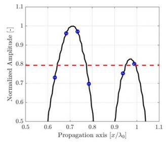
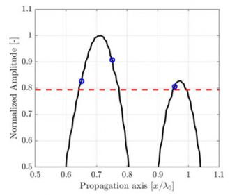
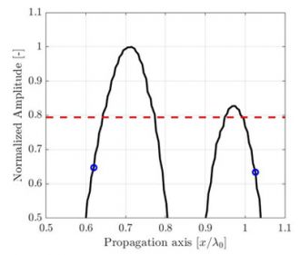
Figure 2. Illustration of the sampling period effect on the recorded amplitude along the propagation axis depicted in Fig. 1. A high-resolution interpolated signal reference (black line) is illustrated to aid the eye. The code compliant amplitude fidelity of 2dB is represented by a red dashed line.
The obvious conclusion is that a denser grid provides a better representation of a continuous signal, as quantified per the AF value from Equation 1, but the optimization problem remains: What is the maximum grid size (Δxmax ) guaranteeing, for all possible grid positions over a TFM image, an amplitude fidelity  that is equal to a target valuee AFtarget? Or,

It is clear from this problem statement that all translations of the grid, identified by displacements (ϵx,ϵy), must be taken into account to obtain the maximum for a fixed cell size (Δx). This is to cover all possible cases of grid placements to compute the TFM image.
In the following section, an illustration of the measurement principle for the set of amplitude fidelity values produced from multiple grid displacements {(Δx)}(ϵx,ϵy) is provided.
Empirical Measurement of Amplitude Fidelity
Before presenting how the amplitude fidelity can be estimated using a simple analytical model, it is of central importance to define how to measure it experimentally in the case of a TFM image. Several techniques have been described and proposed in the NDT industry [10–12], but some of them do not quantify the amplitude fidelity in a complete manner. The empirical measurement of the amplitude fidelity can quickly become an acquisition burden for the NDT technician as it requires the computation of a large number of TFM images from multiple precise TFM grid positions.
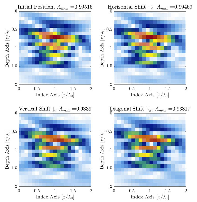
Figure 3. Illustration of the AF variation caused by the discrete grid resolution as the grid is displaced in 3 different directions. The grid resolution is set to Δx=Δy=λ0/10. The grid is shifted by one fourth of the grid cell on the right (ϵx=λ0/40,ϵy=0) (top right), bottom (ϵx=0,ϵy=λ0/40) (bottom left), and diagonally (ϵx=λ0/40,ϵy=λ0/40) (bottom right).
For typical TFM applications, an SDH is used as a reference flaw for amplitude calibration and amplitude fidelity measurement [1,10]. The observed amplitude will vary the most along the principal axis of acoustic propagation, which is a function of the probe, wedge, and target position in the region of interest (i.e., the TFM grid position relative to the probe). In the case illustrated in Figure 1, the principal axis of propagation is almost vertical. However, for a generic measurement method, the axis of propagation will be different depending on the location within the region of interest. For a TFM image, the sampling grid must be moved in all directions to capture the true amplitude variation caused by the discrete grid. This process is illustrated below with the same example of Figure 1 (center), which has a grid resolution of λ0/10.
It is suggested to move the grid by a fraction of the grid resolution to be tested (e.g., about one-twentieth of the resolution) in every direction for as many times as it is needed to get grid overlap. This means that in order to cover an offset of one grid resolution in the two orthogonal directions, a total of 202 = 400 displacement steps are required (if using the suggested grid step of one-twentieth of the resolution). The maximum amplitude is recorded for every grid offset, and the maximum and minimum recorded values are used to obtain the amplitude fidelity using Equation 2. In the case presented in Figure 3, the grid resolution is λ0/10, and the measured amplitude fidelity is 0.88 dB. Judging by the number of displacements required, this manual process would be cumbersome and time-consuming for the NDT technician. It also means that a total of 400 TFM images must be computed to measure the amplitude fidelity of a single grid resolution.
It is worth mentioning that by using the software displacement of the TFM grid position relative to the probe instead of a mechanical displacement of the probe relative to the part as proposed in ASME Section V [12], multiple TFM images can be generated using a single FMC data set. One other benefit of this approach is the ability to access the vertical component of the grid. Indeed, the probe and wedge cannot be mechanically moved relative to the selected SDH along the depth axis.
Some NDT devices readily provide semiautomated tools that shift the TFM grid, record the maximum amplitude in the region of interest, and ultimately compute the resulting amplitude fidelity [11]. However, these tools usually only shift the grid in the horizontal direction and consequently underestimate the amplitude fidelity. For comparison, if the grid is moved solely along the horizontal axis, for example, as illustrated in Figure 3, the measured amplitude fidelity is 0.06 dB, which is more than 15 times lower than the amplitude fidelity measured when considering the vertical axis.
A Phenomenological Model for Amplitude Fidelity Estimation
This section proposes a simple analytical model based on empirical observation. The phenomenological model considers the signal behavior along the principal axis of propagation, which is assumed to contain most of the amplitude fluctuations and, therefore, to be the most sensitive to the grid resolution. Figure 4 shows the empirical profile of a resulting TFM image of an SDH along the principal axis of propagation (blue) and along the beam waist axis (red). The origin of the axis is located at the apparent maximum amplitude location of the envelope representation, which explains the small offset along the axis  for the oscillatory representation. The profiles for the standard oscillatory TFM and for the envelope of the TFM are provided.
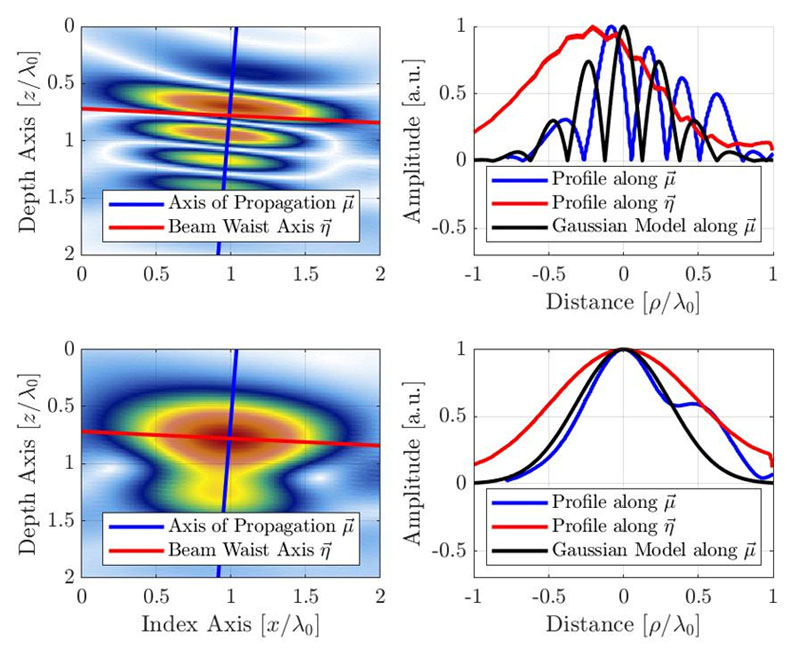
Figure 4. TFM image (top: oscillatory, bottom: envelope) with the signal profile along the acoustic propagation axis and the beam waist axis. The proposed Gaussian model is also illustrated for the oscillatory and envelope TFM images. Note the apparent wavelength is halved because of the pulse-echo nature of the TFM beamforming.
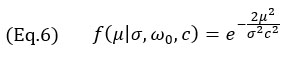
As stated previously, the axis of greatest amplitude variation is assumed to be along the principal axis of acoustic propagation. The model hence aims to reproduce the amplitude variation in this direction. The model signal is a cosine modulated Gaussian
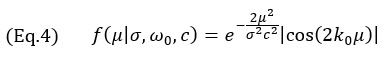
where k0=ω0/c is the wavenumber at the central angular frequency ω0 of the probe, σ is the width parameter dependent on the central frequency and the relative bandwidth bw. The width parameter σ is computed using
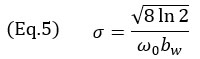
For a typical NDT phased array probe, the relative bandwidth is near the 60% mark, hence a value of (bw=0.6) is used in the model. This, in turn, makes the Gaussian envelope larger than a single cosine oscillation. It is worth mentioning that the central frequency of the cosine term in Equation 3 is doubled from the probe central frequency. This is due to the pulse-echo nature of the TFM imaging (transmitting and receiving path) and can be observed in the distance between oscillations in Figure 4. In fact, the conversion between the time domain and the space domain is written as μ = tc/2. It also explains the factor 2 used as the exponential term of Equation 3.
For the oscillatory model of Equation 4, since the Gaussian envelope is much larger than a single oscillation of the cosine function, only the values |μ|≤λ0/8 are considered, as larger values produce spatial aliasing for the AF.
For the TFM envelope model, only the Gaussian term of Equation 4 is used, yielding the following
which is valid for any grid resolution. The profile obtained with the model of Equations 3 and 7 is illustrated in Figure 4 alongside the experimental profiles. Note the empirical measurements also show the surface wave signal (the “wrap around” echo typical of SDHs) lagging behind the main echo, a feature that is noticeably absent from the proposed model.
The orientation of the flaw relative to the grid orthogonal axes must be considered in order to obtain the amplitude fidelity worst-case scenario with the model. As illustrated in Figure 5a, the worst-case scenario for the oscillatory TFM occurs when the principal axis of acoustic propagation is parallel to one of the grid axes. Hence, the amplitude fidelity must be computed as if the maximum amplitude is centered between two grid point along either axis  or
or  , yielding

for Δx≤λ0/4. For the TFM envelope, the worst-case scenario occurs when the amplitude profile is identical along the principal axis of propagation and the beam waist axis  . This case—illustrated in Figure 5b—corresponds to when the SDH is represented as a circle, and, hence, the principal axis of propagation can have any orientation. The worst-case scenario occurs when the SDH echo is centered between four adjacent points, as illustrated. In this case, the amplitude fidelity must be computed along the grid diagonal, effectively yielding

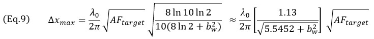
An approximate form for the value of Δx with respect to AF, in cases where the AF value is small, which is the typical use case for NDT applications, may be obtained for the oscillatory model of Equation 7,
and the envelope model of Equation 8,
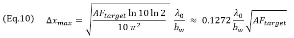
These expressions translate the square root dependency of the grid size on the AF value in all cases. Equation 9 was obtained using the second-order Taylor’s series approximation of Equation 7. This approximation is illustrated in Figure 6 alongside the exact model. Also, note that the grid size for the oscillating model is almost independent of the relative bandwidth for small bw. It is also worth mentioning that, both for the oscillating and envelope models, the maximum grid resolution Δxmax is related to the square root of the targeted amplitude fidelity. These values represent the maximum grid resolution for code compliance based on the phenomenological model.
(a) Worst-case scenario for the oscillatory TFM occurs when axis |
(b) Worst-case scenario for the TFM envelope occurs when the amplitude profile along |
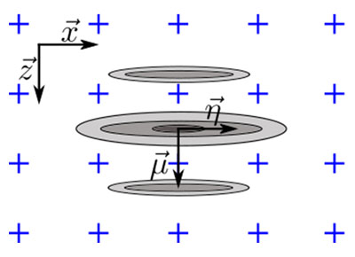
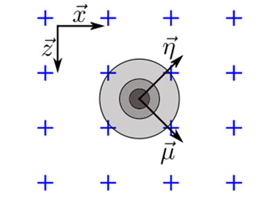
Figure 5. Illustration of the flaw orientation relative to the grid orthogonal axis for the worst-case scenario, for (a) the oscillatory TFM and (b) the TFM envelope.
Experimental Validation
The proposed model is validated with the empirical results on three different TFM inspection use cases. For all three TFM setups, several SDHs were imaged with various grid resolutions, and the amplitude fidelity was measured using the method described previously. The parameters of the three use cases are described in Table 1. The first case is in contact with a high-frequency probe (7.5 MHz), the second use case uses shear waves at a lower frequency (5 MHz), and the third use case uses shear waves at a higher probe frequency (10 MHz) and element counts. For all cases, the SDHs are located within 50 mm from the top surface of a carbon steel block.
Table 1: Parameters of the TFM setups used for the amplitude fidelity experimental validation.
| Case | Probe Parameters | Wedge Parameters | Part Parameters | TFM Mode | |||||
|---|---|---|---|---|---|---|---|---|---|
|
Frequency
[MHz] |
Number
[#] |
Pitch
[mm] |
Velocity
[m/s] |
Angle
[°] |
Height
[mm] |
Velocity
cp - cs [m/s] |
SDH
Diameter [mm] | ||
| 1 | 7.5 | 64 | 1.0 | n/a | n/a | 0 | 3240 - 5890 | 1 | L-L |
| 2 | 5 | 32 | 1.0 | 2330 | 36.1 | 11.0 | 3240 - 5890 | 0.5 | T-T |
| 3 | 10 | 64 | 0.5 | 2330 | 36.1 | 11.0 | 3240 - 5890 | 1 | T-T |
Figure 5 shows the resulting amplitude fidelity for the standard oscillatory TFM (top) and for the TFM envelope (bottom). Each individual gray point represents a different combination of use case, SDHs, and grid resolution. The amplitude fidelity estimated using the Gaussian model presented previously is shown with a black plain curve. The red dashed line represents the code-compliance limit of 2 dB.
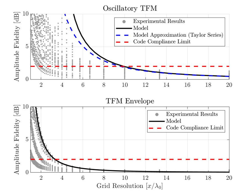
Figure 6. Comparison between empirical amplitude fidelity measurements and proposed Gaussian model results for the standard oscillatory TFM (top) and for the TFM envelope (bottom).
With the proposed model, the resolution needed to be code compliant is λ0/9.9 for the oscillatory TFM and λ0/3.3 for the TFM envelope. Experimental results show that the minimal grid resolution for code compliance is around λ0/10 for the standard oscillatory TFM and λ0/3.3 for the TFM envelope. Note, however, that those values were taken from the worst experimental case presented. Some of the measured amplitude fidelity values are below 2 dB, even with a coarser grid resolution. Therefore, the proposed model provides good, yet conservative estimates for the amplitude fidelity of a TFM setup.
Conclusion
The amplitude fidelity of a TFM setup is an important measure of the imaging robustness with regards to the grid resolution. The denser the grid, the lower the amplitude fidelity value. Codes and standards now include the total focusing method as a new inspection technique and require the amplitude fidelity to be 2 dB or less. This paper presents how the amplitude fidelity can be correctly measured empirically and proposes a simple analytical model to estimate the amplitude fidelity of the results for a TFM setup.
A simple analytical model was proposed based on the amplitude profile along the principal axis of acoustic propagation. The model estimates the amplitude profile as a Gaussian modulated cosine oscillation. Using this profile to estimate the amplitude fidelity leads to good results for both the standard oscillatory TFM and the TFM envelope. Empirical results showed the need for a grid resolution of up to λ0/10 or λ0/3.3, respectively, for the standard oscillatory TFM and the TFM envelope. The proposed analytical model estimates the need for a grid resolution of λ0/9.9 for the standard TFM and λ0/3.3 for the TFM envelope. The proposed model could, therefore, be used to estimate the amplitude fidelity of TFM setup.
To learn more about the benefits of using the TFM envelope as part of a code-compliant solution, read the white paper “Use of the Total Focusing Method with the Envelope Feature.”
Bibliography
[1] ASME Committee, 2019, “ASME BPVC.V Article 4 Mandatory Appendix XI Full Matric Capture.”
[2] Oralkan, O., Ergun, A. S., Johnson, J. A., Karaman, M., Demirci, U., Kaviani, K., Lee, T. H., and Khuri-Yakub, B. T., 2002, “Capacitive Micromachined Ultrasonic Transducers: Next-Generation Arrays for Acoustic Imaging?,” IEEE Trans. Ultrason., Ferroelect., Freq. Contr., 49(11), pp. 1596–1610.
[3] Thomenius, K. E., 1996, “Evolution of Ultrasound Beamformers,” 1996 IEEE Ultrasonics Symposium. Proceedings, IEEE, San Antonio, TX, USA, pp. 1615–1622.
[4] Freeman, S., Li, P., and O’Donnell, M., “Retrospective Dynamic Transmit Focusing,” p. 24.
[5] Wilcox, P. D., 2006, “Exploiting the Full Data Set from Ultrasonic Arrays by Post-Processing,” AIP Conference Proceedings, AIP, Brunswick, Maine (USA), pp. 845–852.
[6] Portzgen, N., Gisolf, D., and Blacquiere, G., 2007, “Inverse Wave Field Extrapolation: A Different NDI Approach to Imaging Defects,” IEEE Transactions on Ultrasonics, Ferroelectrics and Frequency Control, 54(1), pp. 118–127.
[7] Sharpe, R. S., ed., 1982, Research Techniques in Nondestructive Testing. Vol. 6: ..., Acad. Press, London.
[8] Holmes, C., Drinkwater, B. W., and Wilcox, P. D., 2008, “Advanced Post-Processing for Scanned Ultrasonic Arrays: Application to Defect Detection and Classification in Non-Destructive Evaluation,” Ultrasonics, 48(6–7), pp. 636–642.
[9] Holmes, C., Drinkwater, B. W., and Wilcox, P. D., 2005, “Post-Processing of the Full Matrix of Ultrasonic Transmit–Receive Array Data for Non-Destructive Evaluation,” NDT & E International, 38(8), pp. 701–711.
[10] ISO, 2020, “ISO/DIS 23865 -FMC-TFM - General Use of TFM-FMC Technique.”
[11] Johnson, P., 2019, “With a New Software Wizard, There’s No Sorcery but the Magic of the M2M Gekko Is Evident with Instant Code Compliance for Your TFM Weld Inspections.,” Code Compliant TFM Weld Inspection with Three Clicks.
[12] ASME Committee, 2019, “ASME BPVC.V Article 4 Nonmandatory Appendix F - Examination of Welds Using Full Matrix Capture.”